ex2-logistic regression

AndrewNg 机器学习习题ex2-logistic regression

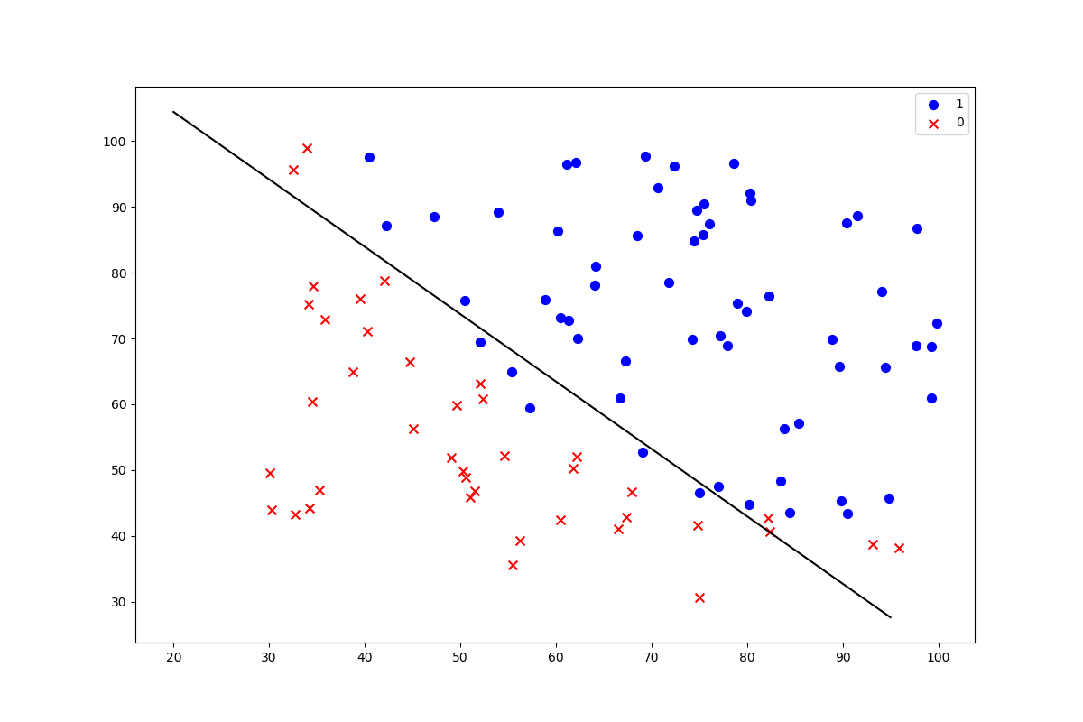
练习数据ex2data1.txt和ex2data2.txt都是由三列数字组成的文本文件，前两列是特征，第三列是结果，结果只有0和1两种。

浏览数据

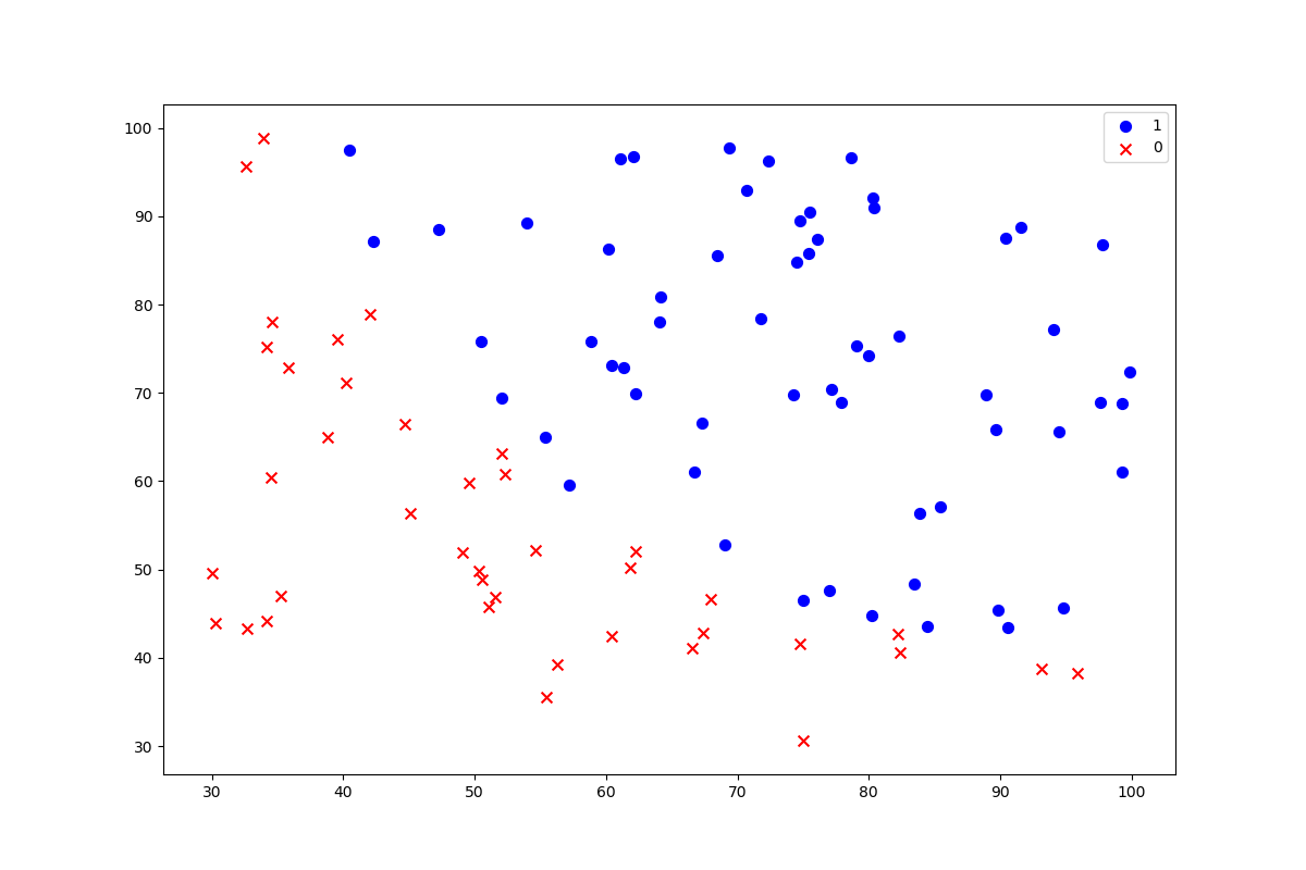
画出散点图，观察两个不同结果的分类情况，有明显的决策边界。

import numpy as np
import pandas as pd
import matplotlib.pyplot as plt

path = './data/ex2data1.txt'
names=['exam 1', 'exam 2', 'admitted']
data = pd.read_csv(path, header=None, names=names)
print(data.head())


# 可视化
def data_visual(data, names, theta=None):
    positive = data[data[names[2]].isin([1])]
    negative = data[data[names[2]].isin([0])]
    fig, ax = plt.subplots(figsize=(12, 8))
    ax.scatter(positive[names[0]], positive[names[1]], s=50, c='b', marker='o', label='1')
    ax.scatter(negative[names[0]], negative[names[1]], s=50, c='r', marker='x', label='0')
    ax.legend()

    if theta is not None:
        x1 = np.arange(20, 100, 5)
        x2 = (- theta[0] - theta[1] * x1) / theta[2]
        plt.plot(x1, x2, color='black')

    plt.show()


data_visual(data, names)

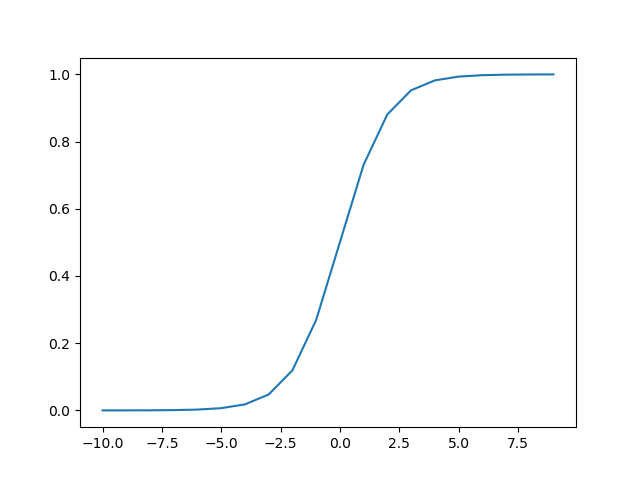
激活函数

逻辑回归模型的假设是： $h_{θ} (x) = g (θ^{T} X)$ 其中： $X$ 代表特征向量 $g$ 代表逻辑函数（logistic function)是一个常用的逻辑函数为S形函数（Sigmoid function），公式为： $g (z) = \frac{1}{1 + e^{- z}}$ 。

# sigmoid函数
def sigmoid(z):
    return 1 / (1 + np.exp(-z))


# 检查激活函数
def sigmoid_visual():
    nums = np.arange(-10, 10, step=1)
    plt.plot(nums, sigmoid(nums))
    plt.show()


sigmoid_visual()

代价函数与预处理

代价函数：

$J (θ) = \frac{1}{m} \sum_{i = 1}^{m} [- y^{(i)} \log (h_{θ} (x^{(i)})) - (1 - y^{(i)}) \log (1 - h_{θ} (x^{(i)}))]$

# 代价函数
def cost(theta, X, Y):
    theta = np.matrix(theta)
    X = np.matrix(X)
    Y = np.matrix(Y)
    first = np.multiply(-Y, np.log(sigmoid(X * theta.T)))
    second = np.multiply((1 - Y), np.log(1 - sigmoid(X * theta.T)))
    return np.sum(first - second) / len(X)


# 数据预处理
# add a ones column - this makes the matrix multiplication work out easier
data.insert(0, 'Ones', 1)

# set X (training data) and y (target variable)
cols = data.shape[1]
X = data.iloc[:, 0: cols - 1]
Y = data.iloc[:, cols - 1: cols]

# convert to numpy arrays and initalize the parameter array theta
X = np.array(X.values)
Y = np.array(Y.values)
theta = np.zeros(3)

# 检查维度
print(X.shape, theta.shape, Y.shape)  # (100, 3) (3,) (100, 1)
print(cost(theta, X, Y))  # 初始值的代价

初始化的代价函数值为：0.6931471805599453

梯度下降

$\frac{\partial J (θ)}{\partial θ_{j}} = \frac{1}{m} \sum_{i = 1}^{m} (h_{θ} (x^{(i)}) - y^{(i)}) x_{_{j}}^{(i)}$

# 梯度下降
def gradient(theta, X, Y):
    theta = np.matrix(theta)
    X = np.matrix(X)
    y = np.matrix(Y)

    parameters = int(theta.ravel().shape[1])
    grad = np.zeros(parameters)

    error = sigmoid(X * theta.T) - Y

    for i in range(parameters):
        term = np.multiply(error, X[:, i])
        grad[i] = np.sum(term) / len(X)


    return grad

训练数据与决策边界

# 用SciPy's truncated newton（TNC）实现寻找最优参数
result = opt.fmin_tnc(func=cost, x0=theta, fprime=gradient, args=(X, Y))
print(result)
print(cost(result[0], X, Y))

theta = result[0]
# 画出决策边界
data_visual(data, names, theta)


# 计算预测效果
def predict(theta, X):
    probability = sigmoid(X * theta.T)
    return [1 if x >= 0.5 else 0 for x in probability]


theta_min = np.matrix(result[0])
predictions = predict(theta_min, X)
correct = [1 if ((a == 1 and b == 1) or (a == 0 and b == 0)) else 0 for (a, b) in zip(predictions, Y)]
accuracy = (sum(map(int, correct)) % len(correct))
print('accuracy = {}%'.format(accuracy))

accuracy = 89%

逻辑回归正则化

path2 = './data/ex2data2.txt'
names = ['test1', 'test2', 'accepted']
data2 = pd.read_csv(path2, header=None, names=names)
print(data2.head())

#data_visual(data2, names)

degree = 5
x1 = data2['test1']
x2 = data2['test2']

data2.insert(3, 'Ones', 1)

for i in range(1, degree):
    for j in range(0, i):
        data2['F' + str(i) + str(j)] = np.power(x1, i-j) * np.power(x2, j)

data2.drop('test1', axis=1, inplace=True)
data2.drop('test2', axis=1, inplace=True)

print(data2.head())

# 正则化代价函数 learng_rate = λ lambda
def cost_reg(theta, X, Y, learng_rate):
    theta = np.matrix(theta)
    X = np.matrix(X)
    Y = np.matrix(Y)

    first = np.multiply(-Y, np.log(sigmoid(X * theta.T)))
    second = np.multiply((1 - Y), np.log(1 - sigmoid(X * theta.T)))
    reg = (learng_rate / (2 * len(X))) * np.sum(np.power(theta[:, 1: theta.shape[1]], 2))

    return np.sum(first - second) / len(X) + reg


def gradient_reg(theta, X, Y, learng_rate):
    theta = np.matrix(theta)
    X = np.matrix(X)
    Y = np.matrix(Y)

    parameters = int(theta.ravel().shape[1])
    grad = np.zeros(parameters)

    error = sigmoid(X * theta.T) - Y

    for i in range(parameters):
        term = np.multiply(error, X[:, i])

        if(i == 0):
            grad[i] = np.sum(term) / len(X)
        else:
            grad[i] = (np.sum(term) / len(X)) + ((learng_rate / len(X)) * theta[:, i])

    return grad

# set X and y (remember from above that we moved the label to column 0)
cols = data2.shape[1]
X2 = data2.iloc[:,1:cols]
Y2 = data2.iloc[:, :1]

# convert to numpy arrays and initalize the parameter array theta
X2 = np.array(X2.values)
Y2 = np.array(Y2.values)
theta2 = np.zeros(11)

learng_rate = 1

print(cost_reg(theta2, X2, Y2, learng_rate))
print(gradient_reg(theta2, X2, Y2, learng_rate))

result2 = opt.fmin_tnc(func=cost_reg, x0=theta2, fprime=gradient_reg, args=(X2, Y2, learng_rate))
print(result2)

theta_min = np.matrix(result2[0])
predictions = predict(theta_min, X2)
correct = [1 if ((a == 1 and b == 1) or (a == 0 and b == 0)) else 0 for (a, b) in zip(predictions, Y2)]
accuracy = (sum(map(int, correct)) % len(correct))
print('accuracy = {0}%'.format(accuracy))

accuracy = 78%

正则化画出决策边界

import numpy as np
import pandas as pd
import matplotlib.pyplot as plt
import scipy.optimize as opt
import seaborn as sns


def get_y(df):  # 读取标签
#     '''assume the last column is the target'''
    return np.array(df.iloc[:, -1])  # df.iloc[:, -1]是指df的最后一列


def sigmoid(z):
    return 1 / (1 + np.exp(-z))


def gradient(theta, X, y):
#     '''just 1 batch gradient'''
    return (1 / len(X)) * X.T @ (sigmoid(X @ theta) - y)


def cost(theta, X, y):
    ''' cost fn is -l(theta) for you to minimize'''
    return np.mean(-y * np.log(sigmoid(X @ theta)) - (1 - y) * np.log(1 - sigmoid(X @ theta)))


df = pd.read_csv('./data/ex2data2.txt', names=['test1', 'test2', 'accepted'])
df.head()


def feature_mapping(x, y, power, as_ndarray=False):
#     """return mapped features as ndarray or dataframe"""
    # data = {}
    # # inclusive
    # for i in np.arange(power + 1):
    #     for p in np.arange(i + 1):
    #         data["f{}{}".format(i - p, p)] = np.power(x, i - p) * np.power(y, p)

    data = {"f{}{}".format(i - p, p): np.power(x, i - p) * np.power(y, p)
                for i in np.arange(power + 1)
                for p in np.arange(i + 1)
            }

    if as_ndarray:
        return pd.DataFrame(data).as_matrix()
    else:
        return pd.DataFrame(data)


x1 = np.array(df.test1)
x2 = np.array(df.test2)
data = feature_mapping(x1, x2, power=6)
print(data.shape)
print(data.head())


theta = np.zeros(data.shape[1])
X = feature_mapping(x1, x2, power=6, as_ndarray=True)
print(X.shape)

y = get_y(df)
print(y.shape)


def regularized_cost(theta, X, y, l=1):
#     '''you don't penalize theta_0'''
    theta_j1_to_n = theta[1:]
    regularized_term = (l / (2 * len(X))) * np.power(theta_j1_to_n, 2).sum()

    return cost(theta, X, y) + regularized_term
# 正则化代价函数


regularized_cost(theta, X, y, l=1)


def regularized_gradient(theta, X, y, l=1):
#     '''still, leave theta_0 alone'''
    theta_j1_to_n = theta[1:]
    regularized_theta = (l / len(X)) * theta_j1_to_n

    # by doing this, no offset is on theta_0
    regularized_term = np.concatenate([np.array([0]), regularized_theta])

    return gradient(theta, X, y) + regularized_term


print('init cost = {}'.format(regularized_cost(theta, X, y)))

res = opt.minimize(fun=regularized_cost, x0=theta, args=(X, y), method='Newton-CG', jac=regularized_gradient)


def draw_boundary(power, l):
#     """
#     power: polynomial power for mapped feature
#     l: lambda constant
#     """
    density = 1000
    threshhold = 2 * 10**-3

    final_theta = feature_mapped_logistic_regression(power, l)
    x, y = find_decision_boundary(density, power, final_theta, threshhold)

    df = pd.read_csv('./data/ex2data2.txt', names=['test1', 'test2', 'accepted'])
    sns.lmplot('test1', 'test2', hue='accepted', data=df, size=6, fit_reg=False, scatter_kws={"s": 100})

    plt.scatter(x, y, c='R', s=10)
    plt.title('Decision boundary')
    plt.show()


def feature_mapped_logistic_regression(power, l):
#     """for drawing purpose only.. not a well generealize logistic regression
#     power: int
#         raise x1, x2 to polynomial power
#     l: int
#         lambda constant for regularization term
#     """
    df = pd.read_csv('./data/ex2data2.txt', names=['test1', 'test2', 'accepted'])
    x1 = np.array(df.test1)
    x2 = np.array(df.test2)
    y = get_y(df)

    X = feature_mapping(x1, x2, power, as_ndarray=True)
    theta = np.zeros(X.shape[1])

    res = opt.minimize(fun=regularized_cost,
                       x0=theta,
                       args=(X, y, l),
                       method='TNC',
                       jac=regularized_gradient)
    final_theta = res.x

    return final_theta


def find_decision_boundary(density, power, theta, threshhold):
    t1 = np.linspace(-1, 1.5, density)
    t2 = np.linspace(-1, 1.5, density)

    cordinates = [(x, y) for x in t1 for y in t2]
    x_cord, y_cord = zip(*cordinates)
    mapped_cord = feature_mapping(x_cord, y_cord, power)  # this is a dataframe

    inner_product = mapped_cord.as_matrix() @ theta

    decision = mapped_cord[np.abs(inner_product) < threshhold]

    return decision.f10, decision.f01


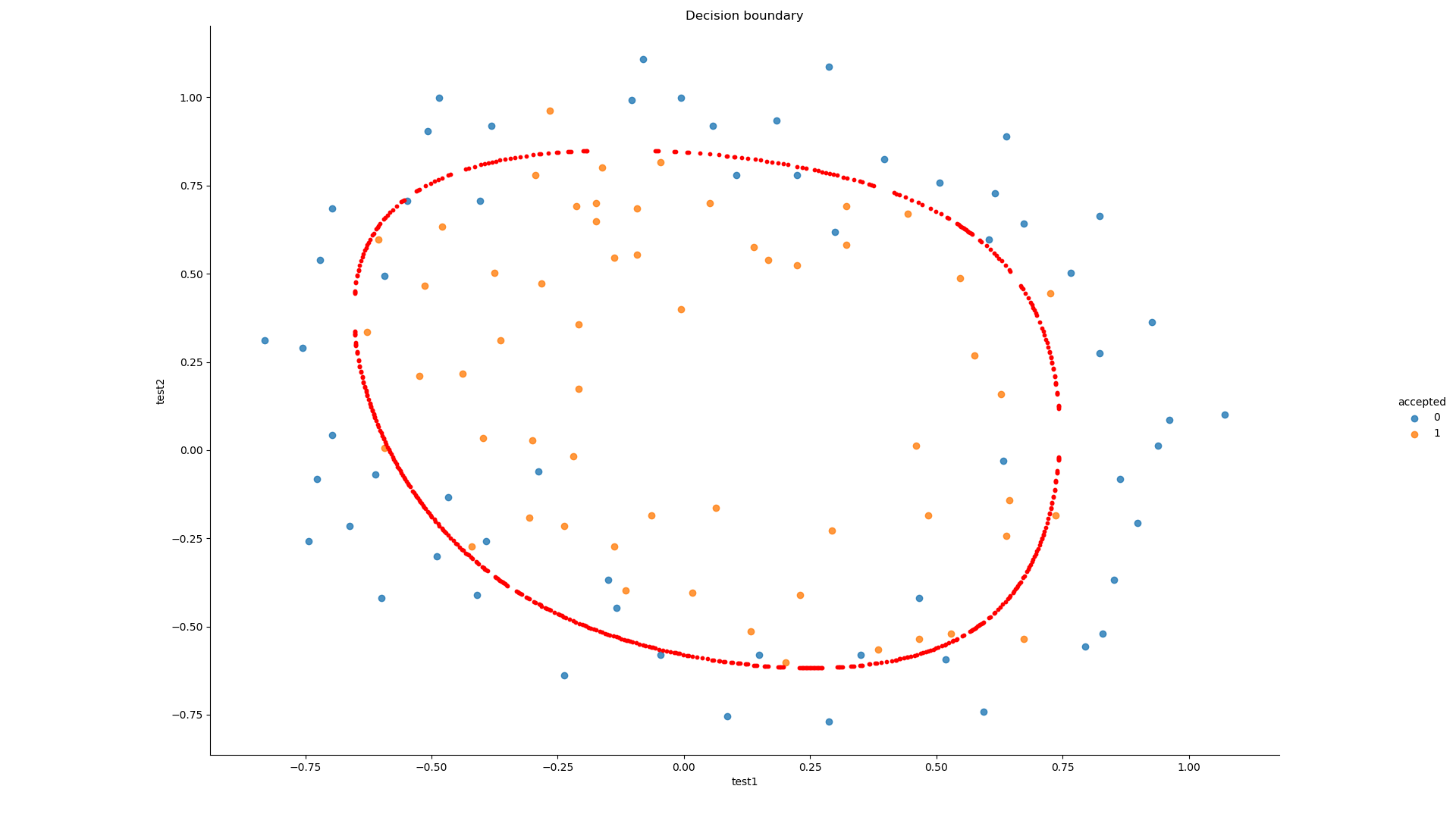
# 寻找决策边界函数
draw_boundary(power=6, l=1)  # lambda=1
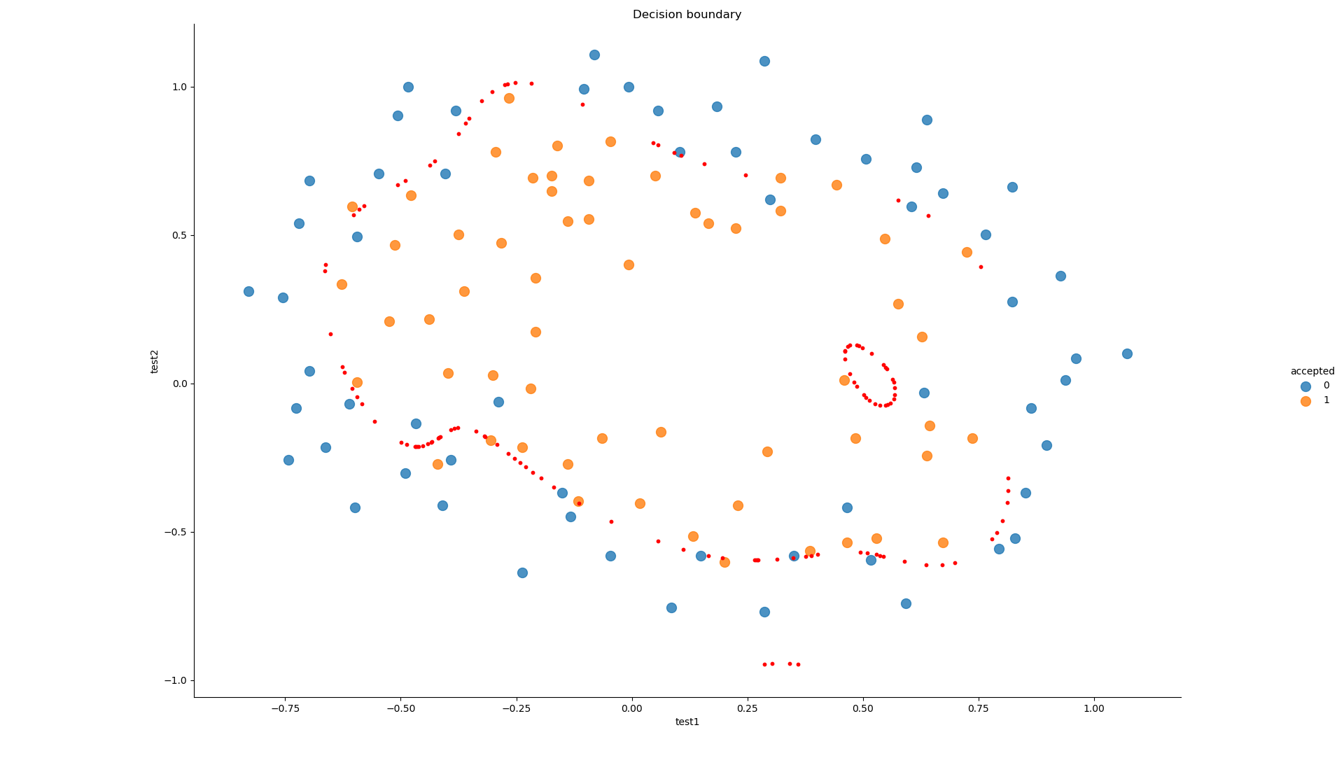
draw_boundary(power=6, l=0)  # lambda=1 过拟合
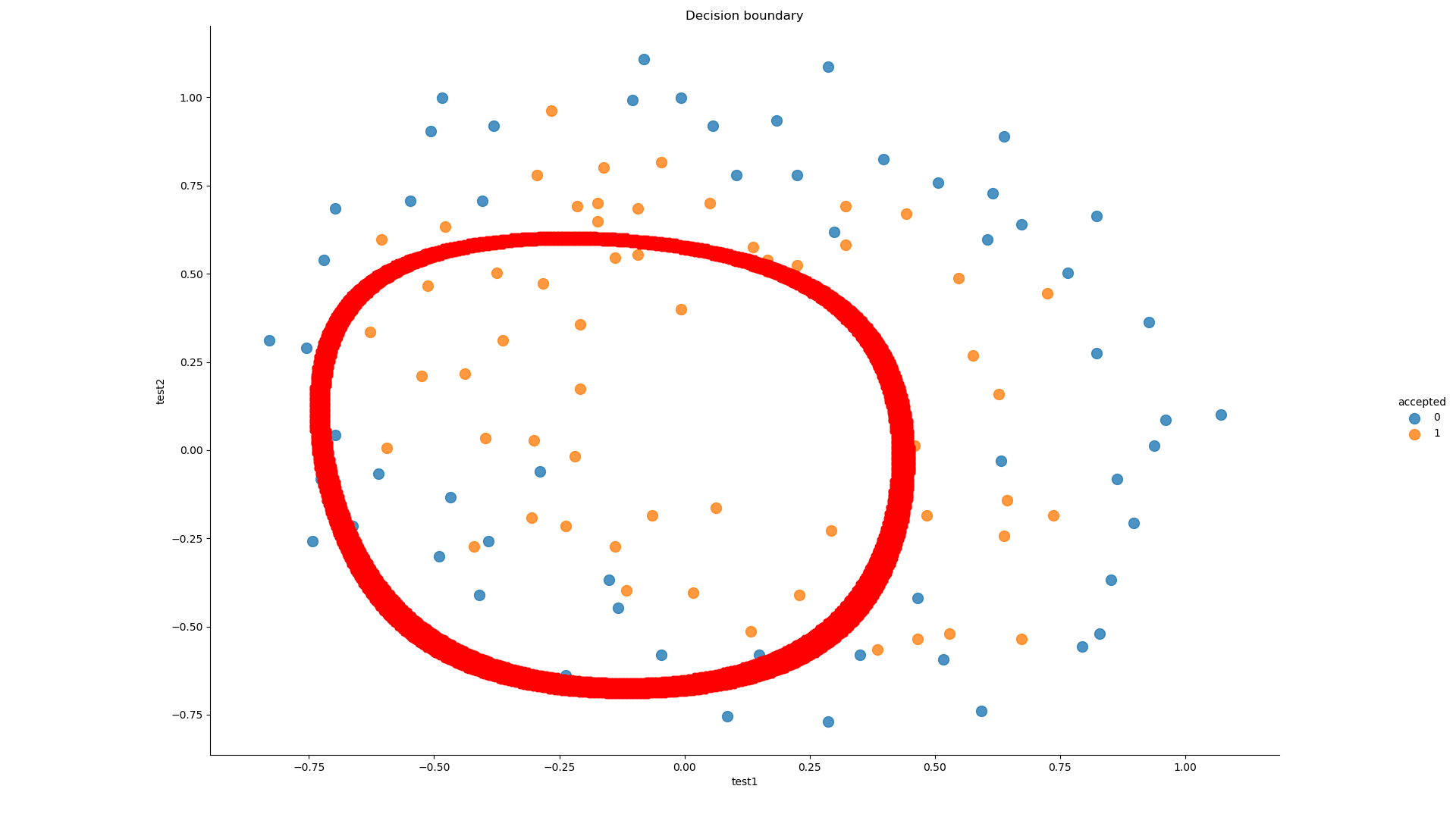
draw_boundary(power=6, l=100)  # lambda=1 欠拟合